Journal Articles
| Browse in : |
All
> Journals
> Overload
> 90
(8)
All > Topics > Design (236) Any of these categories - All of these categories |
Note: when you create a new publication type, the articles module will automatically use the templates user-display-[publicationtype].xt and user-summary-[publicationtype].xt. If those templates do not exist when you try to preview or display a new article, you'll get this warning :-) Please place your own templates in themes/yourtheme/modules/articles . The templates will get the extension .xt there.
Title: If You Can't See Me, I Can't See You
Author: webeditor
Date: 06 May 2009 09:57:00 +01:00 or Wed, 06 May 2009 09:57:00 +01:00
Summary: Knowing where the doors are is only the start. Stuart Golodetz works out what he can see through them.
Body:
In my last article, I talked about how to generate a set of portals (doorways) in a 3D world using a BSP tree. These portals can be very useful on their own (e.g. it's possible to write a portal engine), but they also have an application in determining a potential visibility relation between the empty leaves of the BSP tree, and it's that application that I will discuss in this article.
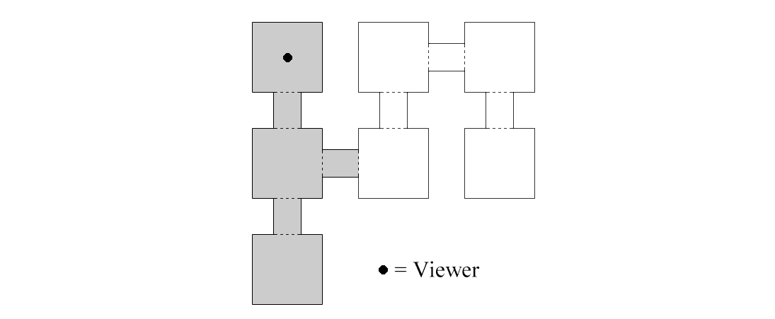
One of the early challenges faced when writing a 3D engine is how to avoid rendering your entire level when you can only see a small bit of it, since this slows your frame-rate to a crawl. This was a serious problem for the developers of the original Quake [Abrash] . The solution eventually adopted by id Software's John Carmack (and thereby popularized) was to precompute the set of empty leaves potentially visible from each empty leaf (also known as the PVS, or potentially visible set, of each leaf), using a method originally described in [Teller] . This solves the scale problem and allows you to have large levels with a high frame-rate (of course, it still doesn't mean that you can have large numbers of polygons all in the same room and maintain your frame-rate, but that's an entirely separate challenge). The idea is essentially that once the potentially visible sets for each leaf have been calculated, you can get away with rendering only the polygons in the leaves which are in the PVS of the current viewer's leaf: in other words, you render only the polygons that can potentially be seen from somewhere in the current room in which the viewer resides. This greatly reduces the number of polygons that need to be rendered each frame (see Figure 1: only the grey leaves need to be rendered from the specified viewer position).
|
| Figure 1 |
Door-to-door
The challenge here is in how to calculate the PVS in the first place. Clearly, since it's computed offline, we could theoretically sit down for each level and fill in the O(n2) entries by hand, but this isn't a very attractive proposition when n (the number of empty leaves in the level) is even moderately large.
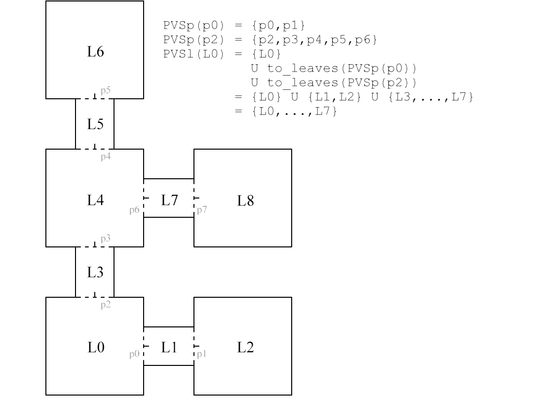
The method we use in practice involves the portals we generated last time. We observe that each leaf can potentially see the union of what its outgoing portals can potentially see: in other words, if I'm standing somewhere arbitrary in a room, I can potentially see exactly what can potentially be seen from all the openings (doorways, windows, skylights, etc.) leading out of that room. The leaf-to-leaf visibility problem can thereby be reduced to a portal-to-portal visibility problem (see Figure 2: note that only the portals relevant to the example have been shown), and it turns out that there is a direct method for generating a portal-to-portal visibility relation.
|
| Figure 2 |
Antipenumbrae
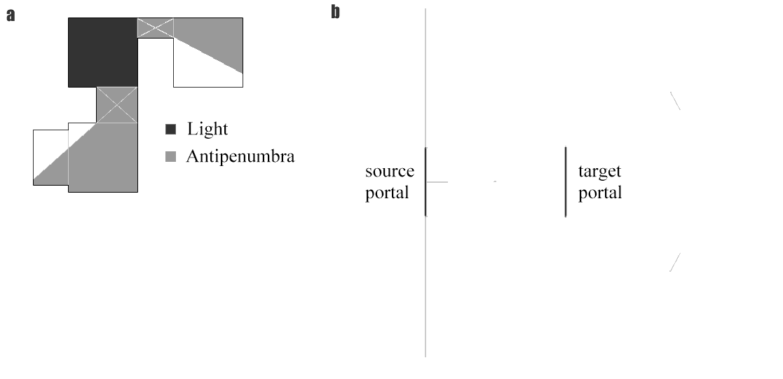
The basic idea is shown in Figure 3. We imagine the source leaf as a volume light source, and note that its antipenumbra is the volume in which it can be partially seen (see Figure 3a). For our purposes, however, we will define an antipenumbra as a set of clip planes separating two portals (see Figure 3b): the analogy is obvious, but the latter definition is a more practically useful one.
|
| Figure 3 |
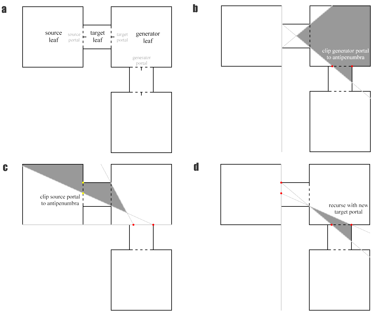
To calculate the (portal) PVS for a given source portal (see Figure 4a), we start by considering all the target portals leading out of its neighbour leaf, i.e. the leaf into which it points (for example, the neighbour leaf of the source portal is the target leaf here). We add any target portal that can be seen from the source portal to the source portal's PVS, and use it to build an antipenumbra which represents the volume that can be seen from the source leaf through the source and target portals. Next, we clip the (outgoing) portals of the target portal's neighbour leaf (the generator leaf) to this volume (see Figure 4b). If a generator portal is not entirely clipped out of existence by this process, then we build a reverse antipenumbra from the generator portal to the target portal (see Figure 4c), and try and clip the source portal to that (this is an optimization that may allow us to clip further bits off our portals and speed up the algorithm). If the source portal is not entirely clipped out of existence either, then we add the generator portal to the source portal's PVS and recurse, using the generator portal as the new target portal (see Figure 4d).
|
| Figure 4 |
Despite its recursive nature, the implementation of this algorithm is actually easier if done iteratively (see Listing 1). We store a stack of portal triples, (source, inter, target), where the inter portal is the portal that was the target when the target portal was the generator. When initialising the stack with the visible portals from the original target leaf, of course, these intermediate portals do not exist, so we just use null (the intermediate portals are actually only an optimization, in any case).
    /**
    Calculates the set of portals that are potentially visible
    from the specified portal, and updates the portal visibility
    table accordingly.

    @param originalSource
    The portal for which to calculate the PVS
    */
    void VisCalculator::calculate_portal_pvs(
       const Portal_Ptr& originalSource)
    {
      int originalSourceIndex =
         portal_index(originalSource);
      Plane originalSourcePlane =
         make_plane(*originalSource);
      std::stack<PortalTriple> st;
      // Initialise the stack with triples targeting
      // all the portals that can be seen from the
      // original source. If only part of a target
      // portal can be seen, we simply split it.
      const std::vector<int>& originalCandidates =
        m_portalsFromLeaf[neighbour_leaf(
        originalSource)];
      for(size_t i=0, size=originalCandidates.size();
         i<size; ++i)
      {
        Portal_Ptr target =
           m_portals[originalCandidates[i]];
        int targetIndex = originalCandidates[i];
        if((*m_portalVis)(originalSourceIndex,
           targetIndex) != PV_NO)
        {
          if((*m_classifiers)(originalSourceIndex,
             targetIndex) == CP_STRADDLE)
          {
            target = split_polygon(*target,
               originalSourcePlane).front;
          }
          st.push(PortalTriple(originalSource,
             Portal_Ptr(), target));
          (*m_portalVis)(originalSourceIndex,
             targetIndex) = PV_YES;
        }
      }
      // Run the actual visibility calculation process.
      while(!st.empty())
      {
        PortalTriple triple = st.top();
        Portal_Ptr source = triple.source, inter =
           triple.inter, target = triple.target;
        int targetIndex = portal_index(target);
        st.pop();
        Antipenumbra ap(source, target);
        const std::vector<int>& candidates =
           m_portalsFromLeaf[neighbour_leaf(target)];
        for(size_t i=0, size=candidates.size();
           i<size; ++i)
        {
          Portal_Ptr generator =
             m_portals[candidates[i]];
          int generatorIndex = candidates[i];
          // If this generator portal might be visible
          // from both the intermediate portal (if it
          // exists) and the target portal, then we
          // need to clip it to find out.
          if((!inter || (*m_portalVis)
             (portal_index(inter),
             generatorIndex) != PV_NO) &&
             ((*m_portalVis)(targetIndex,
             generatorIndex) != PV_NO))
          {
            Portal_Ptr clippedGen =
               ap.clip(generator);
            if(clippedGen)
            {
              Antipenumbra reverseAp(
                 clippedGen->flipped_winding(),
                 target);
              Portal_Ptr clippedSrc =
                 reverseAp.clip(source);
              if(clippedSrc)
              {
                 st.push(PortalTriple(clippedSrc,
                    target, clippedGen));
                 (*m_portalVis)(originalSourceIndex,
                    generatorIndex) = PV_YES;
              }
            }
          }
        }
      }
      // Any portals which haven't been definitely
      // marked as potentially visible at this point
      // can't be seen.
      int portalCount =
         static_cast<int>(m_portals.size());
      for(int i=0; i<portalCount; ++i)
      {
        if((*m_portalVis)(originalSourceIndex,i) !=
           PV_YES)
        (*m_portalVis)(originalSourceIndex,i) = PV_NO;
      }
    }
|
| Listing 1 |
Clipping
Having seen the core visibility calculation process, we need to look at how we construct an antipenumbra in the first place, and then clip to it. Constructing an antipenumbra is a relative simple process (see Listing 2). The idea is to add planes which separate the source portal from the target portal. To do this, we consider each edge on the source portal in turn, and iterate through the target vertices until we find a vertex such that the plane of the triangle it makes with the source edge separates the two portals. We then make sure the plane in question is facing away from the source portal and towards the target portal (for consistency: we could have done it the other way round as well), and add it to the list.
    /**
    Constructs an antipenumbra from a source portal to a target portal.
    For each antipenumbral plane p (except the source plane), it
    is guaranteed to be the case that:
    - classify_polygon_against_plane(*source, p)
         == CP_BACK
    - classify_polygon_against_plane(*target, p)
         == CP_FRONT

    @param source    The source portal
    @param target    The target portal
    */
    Antipenumbra::Antipenumbra(
       const Portal_Ptr& source,
       const Portal_Ptr& target)
    {
      m_planes.push_back(make_plane(*source));
      // Note: In both cases here, source lies behind
      // the generated planes and target lies in front
      // of them.
      add_clip_planes(source, target, CP_BACK);
      // add planes from source to target, with source
      // behind them
      add_clip_planes(target, source, CP_FRONT);
      // add planes from target to source, with target
      // in front of them
    }
    /**
    Adds clip planes which separate portal 'from' and portal 'to'.
    The classifier specifies on which side of the generated planes
    portal 'from' should lie.

    @param from                     The from portal
    @param to                       The to portal
    @param desiredFromClassifier    The side of the
                planes on which portal from should lie
    */
    void Antipenumbra::add_clip_planes(
       const Portal_Ptr& from, const Portal_Ptr& to,
       PlaneClassifier desiredFromClassifier)
    {
      int fromCount = from->vertex_count();
      int toCount = to->vertex_count();
      for(int i=0; i<fromCount; ++i)
      {
        const Vector3d& a = from->vertex(i);
        const Vector3d& b = from->vertex(
           (i+1)%fromCount);
        for(int j=0; j<toCount; ++j)
        {
          const Vector3d& c = to->vertex(j);
          Plane_Ptr plane = construct_clip_plane(
             a, b, c);
          if(!plane) continue;
          PlaneClassifier cpFrom =
             classify_polygon_against_plane(*from,
             *plane);
          if(cpFrom == CP_BACK || cpFrom == CP_FRONT)
          {
            PlaneClassifier cpTo =
               classify_polygon_against_plane(*to,
               *plane);
            if((cpTo == CP_BACK || cpTo == CP_FRONT)
               && cpTo != cpFrom)
            {
            // If we get here, either cpFrom ==
            // CP_BACK && cpTo == CP_FRONT, or
            // vice-versa.
              if(cpFrom != desiredFromClassifier)
                 m_planes.push_back(plane->flip());
              else m_planes.push_back(*plane);
                break;
            }
          }
        }
      }
    }
    /**
    Returns the plane through a, b and c.
    @param a    The first vector in the plane
    @param b    The second vector in the plane
    @param c    The third vector in the plane
    @return     As stated
    */
    Plane_Ptr Antipenumbra::construct_clip_plane(
       const Vector3d& a, const Vector3d& b,
       const Vector3d& c)
    {
        Vector3d v1 = b - a;
        Vector3d v2 = c - a;
        Vector3d n = v1.cross(v2);
        if(n.length_squared() < EPSILON)
           return Plane_Ptr();
        return Plane_Ptr(new Plane(n,a));
 }
|
| Listing 2 |
Clipping a portal to an antipenumbra is also relatively straightforward (see Listing 3). All we have to do is classify the portal against each clip plane in turn: if it's behind the plane, it's completely outside the antipenumbra, so we dump it; if it's in front of the plane, we need to carry on clipping it against the other planes; if it straddles the plane, we split it and keep the front half (the bit potentially inside the antipenumbra); if it's on the plane, we treat it as if it were outside the antipenumbra, since it can't be seen properly from the source.
    /**
    Clips the specified polygon to the antipenumbra.

    @param poly     The polygon
    @return         The clipped version of the polygon
    */
    template <typename Vert, typename AuxData>
    shared_ptr<Polygon<Vert,AuxData> >
    Antipenumbra::clip(
       const shared_ptr<Polygon<Vert,AuxData> >& poly)
    {
      typedef Polygon<Vert,AuxData> Poly;
      typedef shared_ptr<Poly> Poly_Ptr;
      Poly_Ptr ret = poly;
      for(std::vector<Plane>::const_iterator it=
         m_planes.begin(), iend=m_planes.end();
         it!=iend; ++it)
      {
         switch(classify_polygon_against_plane(
            *ret, *it))
         {
           case CP_BACK:
           {
             // The polygon is completely outside the
             // antipenumbra.
             return Poly_Ptr();
           }
           case CP_COPLANAR:
           {
             // The polygon lies on the antipenumbra
             // boundary and can't be seen properly
             // from the source.
             return Poly_Ptr();
           }
           case CP_FRONT:
           {
             // Nothing to clip: move onto the next
             // clip plane.
             break;
           }
           case CP_STRADDLE:
           {
              // Split the polygon across the clip plane
             // and keep the bit inside the
             // antipenumbra.
             ret = split_polygon(*ret, *it).front;
             break;
           }
         }
      }
      return ret;
    }
|
| Listing 3 |
Pre-processing
The visibility calculation process is the main part of the algorithm, but before it takes place, we should first construct an initial portal-to-portal vis table to avoid doing lots of redundant work later. At a minimum (see Listing 4), we should fill in entries where:
- Portal i can't see portal j because j is behind or on the plane of i
- Portal i can't see portal j because the two portals are facing each other (portals can only see through the back of other portals).
    /**
    Performs the first phase of the visibility calculation process.
    In this phase, portals which obviously can't see each other (e.g.
    one portal is fully behind another) are marked as such in the
    portal visibility table. This helps avoid a lot of unnecessary
    clipping later on.
    */

    void VisCalculator::initial_portal_vis()
    {
      int portalCount =
         static_cast<int>(m_portals.size());
      m_portalVis.reset(
         new PortalVisTable(portalCount,
         PV_INITIALMAYBE));

      // Calculate the classification relation between
      // the portals. Specifically, classifiers(i,j)
      // will contain the classification of polygon j
      // relative to the plane of i.
      // Note:    This bit could potentially be
      // optimized if we required that portal pairs
      // occupied consecutive indices in the list (e.g.
      // if 1 were necessarily the reverse portal of 0,
      // etc.).
      m_classifiers.reset(
         new ClassifierTable(portalCount));
      for(int i=0; i<portalCount; ++i)
      {
        const Plane plane = make_plane(*m_portals[i]);
        for(int j=0; j<portalCount; ++j)
        {
          if(j == i) (*m_classifiers)(i,j) =
             CP_COPLANAR;
          else (*m_classifiers)(i,j) =
             classify_polygon_against_plane(
             *m_portals[j], plane);
        }
      }

      // Run through the portal visibility table and
      // mark (*m_portalVis)(i,j) as PV_NO if portal
      // i definitely can't see through portal j.
      for(int i=0; i<portalCount; ++i)
      {
        for(int j=0; j<portalCount; ++j)
        {
          if(j == i)
          {
             (*m_portalVis)(i,j) = PV_NO;
             continue;
          }
          // Note: Portals can only see through the
          // back of other portals.
          // If portal j is behind or on the plane of
          // portal i, then i can't see it.
          if((*m_classifiers)(i,j) ==
             CP_BACK || (*m_classifiers)(i,j) ==
             CP_COPLANAR) (*m_portalVis)(i,j) = PV_NO;
          // If portal i is completely in front of
          // portal j, then it's facing i and i can't
          // see through it.
          if((*m_classifiers)(j,i) == CP_FRONT)
             (*m_portalVis)(i,j) = PV_NO;
        }
      }
    }
|
| Listing 4 |
We can do better than this initial portal vis, however, if we next perform a flood fill from each portal (see Listing 5): this allows us to eliminate even more possibilities before we get to the more expensive part of the vis process. These optimizations are essential to make the vis process run in a decent amount of time: without them, it can take ages. Once the flood-filling has taken place, we're ready to run the actual visibility calculation process described initially.
    /**
    Performs the second phase of the visibility calculation process,
    namely flood filling. This is used to refine the initial portal
    visibility table before calculating the final version, the aim
    being to speed up the final calculation process.
    */
    void VisCalculator::flood_fill()
    {
      int portalCount =
         static_cast<int>(m_portals.size());
      for(int i=0; i<portalCount; ++i)
      {
        flood_from(i);
        // If any portals previously thought possible
        // didn't get marked by the flood fill,
        // then they're not actually possible and
        // need to be marked as such.
        for(int j=0; j<portalCount; ++j)
        {
          if((*m_portalVis)(i,j) == PV_INITIALMAYBE)
             (*m_portalVis)(i,j) = PV_NO;
        }
      }
    }

    /**
    Peforms a flood fill from a given portal to refine its approximate
    PVS before it is calculated for real.

    @param originalSource    The portal from which to flood fill
    */
    void VisCalculator::flood_from(int originalSource)
    {
      std::stack<int> st;
      st.push(originalSource);
      while(!st.empty())
      {
        int curPortal = st.top();
        st.pop();
        if(curPortal != originalSource)
           (*m_portalVis)(originalSource, curPortal) =
           PV_FLOODFILLMAYBE;
        int leaf = m_portals[curPortal]
           ->auxiliary_data().toLeaf;
        const std::vector<int>& candidates =
           m_portalsFromLeaf[leaf];
        for(size_t i=0, size=candidates.size();
           i<size; ++i)
        {
          if((*m_portalVis)(originalSource,
             candidates[i]) == PV_INITIALMAYBE)
             st.push(candidates[i]);
        }
      }
    }
|
| Listing 5 |
Post-processing: portal vis to leaf vis
Once the visibility calculations are complete, we have a portal-to-portal visibility table, but what we really need is a leaf-to-leaf table which will tell us which rooms can be seen from which other rooms. To convert the portal vis table to a leaf vis table, we use our earlier observation that a leaf can see precisely the union of whatever its (outgoing) portals can see. The process is slightly complicated by the fact that for implementation reasons, no portal is contained within its own PVS in the code (i.e. portal i can't see itself for coding purposes), but by and large the process is quite simple (see Listing 6). The result is a leaf-to-leaf visibility table we can use to speed up not only in-game rendering, but also lightmapping calculations for static level lighting.
    /**
    Constructs a leaf visibility table from the portal one. The result of the visibility
    calculation process is actually this leaf visibility table, not the portal one, but
    the latter is more convenient during the calculation process itself: we thus convert
    the one to the other once we've finished calculating.
    */
    void VisCalculator::portal_to_leaf_vis()
    {
      const int portalCount = static_cast<int>(m_portals.size());
      m_leafVis.reset( new LeafVisTable(m_emptyLeafCount, LEAFVIS_NO));
      for(int i=0; i<m_emptyLeafCount; ++i)
      {
      // Leaf i can see itself, plus the union of whatever leaves its portals can see.
        (*m_leafVis)(i, i) = LEAFVIS_YES;
        const std::vector<int>& ps = m_portalsFromLeaf[i];
        for(std::vector<int>::const_iterator jt=ps.begin(), jend=ps.end(); jt!=jend; ++jt)
        {
          const int j = *jt;
          // Leaf i can see the leaf pointed to by portal j (even though portal j can't see itself).
          (*m_leafVis)(i, m_portals[j] ->auxiliary_data().toLeaf) = LEAFVIS_YES;
          // Leaf i can see all the leaves pointed to by portals portal j can see.
          for(int k=0; k<portalCount; ++k)
          {
            if((*m_portalVis)(j,k) == PV_YES)
            {
              (*m_leafVis)(i, m_portals[k] ->auxiliary_data().toLeaf) = LEAFVIS_YES;
            }
          }
        }
      }
    }
|
| Listing 6 |
Conclusion
In this article, we've seen how to generate a leaf-to-leaf visibility table for a BSP-based level from a set of portals. This allows us to render larger levels at a reasonable frame-rate. As can be seen from Figure 5, using the PVS approach allows us to render larger levels at a reasonable frame-rate - because we can't possibly see most of the inside of this building, we don't need to render it.
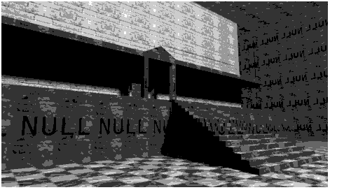
|
| Figure 5 |
References
[Abrash] Graphics Programming Black Book (Special Edition), Mike Abrash, Coriolis Group Books, July 1997.
[Teller] Visibility Computations in Densely Occluded Polyhedral Environments, Seth Teller, PhD Thesis, October 1992.
Notes:
More fields may be available via dynamicdata ..