Journal Articles
| Browse in : |
All
> Journals
> Overload
> 87
(6)
All > Topics > Programming (877) All > Topics > Design (236) Any of these categories - All of these categories |
Note: when you create a new publication type, the articles module will automatically use the templates user-display-[publicationtype].xt and user-summary-[publicationtype].xt. If those templates do not exist when you try to preview or display a new article, you'll get this warning :-) Please place your own templates in themes/yourtheme/modules/articles . The templates will get the extension .xt there.
Title: Seeing Things Differently
Author: webeditor
Date: 26 October 2008 08:59:00 +00:00 or Sun, 26 October 2008 08:59:00 +00:00
Summary: The Multiple Material Marching Cubes (M3C) algorithm builds 3D models from 2D slices. Stuart Golodetz introduces it and provides a C++ implementation.
Body:
Visualizing organs and other features of interest (such as the spine, or tumours, etc.) in 3D is an important process in the medical domain. It makes it much easier for doctors to picture the overall size of a tumour and its relative spatial location if they can see it in 3D, rather than having to try and mentally visualize what's going on after looking through a series of 2D slices. As part of my medical imaging work during my doctorate, I recently spent some time implementing the multiple material marching cubes (M3C) algorithm [Wu03], one of the methods currently used for this process, and (as is often the case when implementing algorithms from research papers, which can only ever give you an overview of the process) the experience turned out to be rather interesting. In my next couple of articles, I'd like to describe not just the algorithm itself (which is probably described more precisely in the original research paper), but how it can be implemented at a code level.
A 3-stage process
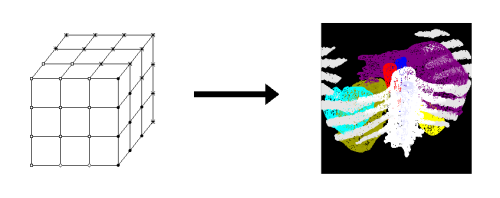
First of all, though, let's discuss the algorithm at a somewhat higher level. M3C takes a labelled volume (grid) of data as input, and produces a coloured triangle mesh as output (see Figure 1).
| M3C converts a labelled volume (left) into a coloured triangle mesh (right). (Note that I've used symbolic rather than numeric labels here for clarity only; the actual labels are numeric. Note also that the labelled volume on the left here is not the actual labelled volume for the mesh on the right, which is huge!) | |
 | |
| Figure 1 | |
Mathematically-speaking, given a label set L = {i | i in [0, n)}, the input is a scalar field f : R3 | [0,X) x [0,Y) x [0,Z) -> L, such that f(x,y,z) indicates the label assigned to grid point (x,y,z). (For example, point (1,2,3) could be labelled with the number 5, which might correspond to the kidney, and indicate that point (1,2,3) should be considered as being inside the kidney.) Such a labelled volume can be constructed, with varying degrees of automation, from a sequence of medical images by a process known as segmentation (something I've referred to in previous articles [Golodetz08]).
The algorithm works in 3 stages: in the first stage, a basic mesh is generated from the volume. This is generally stair-stepped (meaning exactly what it sounds like) and contains far more triangles than it is possible to render at a reasonable frame-rate. The second and third stages thus smooth the mesh (to mitigate the stair-stepping) and decimate it (to drastically reduce the triangle count) respectively.
Stage 1: Basic mesh generation (overview)
The mesh generation process treats the volume as a 3D array of voxels (volume elements) or, to put it another way, as a large number of small cubes. Each label in the volume corresponds to one of the vertices at the points where adjacent cubes meet (as opposed to each voxel having a particular label), thus each cube has 8 labels associated with it, one for each of its vertices (see Figure 2). These labels may all be the same, or all different, or somewhere in between. (In principle, there are thus 88 different combinations which can arise, since there are 8 vertices, and 8 possible label choices per vertex. Note that it doesn't matter that there are more than 8 labels in the entire volume when saying this, since there can only be at most 8 in the same cube at once.)
| Each cube has 8 labels associated with it, one for each of its vertices. |  |
| Figure 2 | |
The mesh is generated on a cube-by-cube basis by adding faces to separate adjacent labels which do not match. This has to be done in a cunning way to ensure that the mesh pieces in adjacent cubes 'match up'. To get a feel for how this process works, we'll first examine the 2D analogue, namely multiple material marching squares (M3S). M3S turns out to be an important subroutine when we repeat the process in 3D, as we'll see later.
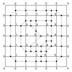
Consider Figure 3a, which shows the result of 'meshing' a 6x6 labelled area in 2D. We treat each square individually, and match it against a set of patterns (see Figure 3b). In each case, the pattern dictates how to mesh the square by (potentially) adding vertices at the midpoints of the square's edges and its centre, and adding mesh edges to join them together. When a vertex is added, it is assigned a set of labels based on the material types it separates. A node at the midpoint of one of the square's edges is assigned the labels of the two corner vertices that edge connects; the centre node (if any) is assigned all the labels present in the square. The mesh piece for each square will contain between 0 and 5 vertices (there are 4 midpoints, plus the square centre) and between 0 and 4 mesh edges. Note that adjacent squares share the midpoint vertices: they can be thought of as belonging to the square edge rather than the square itself.
 |
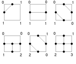 | |
| Meshing a 6x6 labelled area in 2D (left) using the patterns shown (right). The patterns show (top-to-bottom, left-to-right) how to handle squares with 2 labels split (1,3); 2 labels split (2,2) opposite; 2 labels split (2,2) diagonal; 3 labels opposite; 3 labels diagonal; and 4 labels. | ||
| Figure 3 | ||
The patterns themselves are mostly straightforward (note that those not explicitly drawn out are derived by symmetry), and adjacent patterns are guaranteed to match up by design. The only tricky point occurs in Case 3 (the top-right pattern), where there is an ambiguity over whether the material labelled 0 or that labelled 1 should remain contiguous. This was a known problem with the single-material marching cubes algorithm, which M3C extends. It is resolved here by partially-ordering the materials and keeping the lower label contiguous; thus 0 has priority over 1 here.
Having seen how M3S works, we are now ready to consider the equivalent in 3D. The idea here is similarly to generate mesh pieces for each cube so that adjacent mesh pieces join up to form a valid mesh. The way we ensure validity is to use M3S (the 2D analogue) to generate patterns on each cube face; we then connect the vertices generated on the cube faces with triangles within each cube. Since the cube faces (and thus the patterns on them) are shared between adjacent cubes, this guarantees that the mesh pieces will join up appropriately.
The trick now is in how to generate the triangles within each cube. Unfortunately, this turns out to be a somewhat intricate process (but at least it's fun!). The first step is to count the number of centre nodes that have been created by M3S on the cube faces. There are three distinct cases with which to deal: 0 such nodes, 2, or more than 2 (Wu proved in his dissertation that there can't be exactly one face-centred node). The goal in all cases is to try and determine a number of node loops (see Figure 4) that we can then triangulate, as we'll see shortly.
| An example showing a cube with two node loops (based on Figure 6b in [Wu03]: see that paper for further examples). | 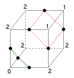 |
| Figure 4 | |
In the case of 0 face-centred nodes, we don't need to do anything special. The nodes and edges added by M3S already form closed loops, and their nodes share the same labels. The situation is more complicated when there are two or more face-centred nodes. In the former situation, we need to add an edge between the two face-centred nodes to form the node loops (see Figure 5). The loops are then distinguished by the fact that there are exactly two labels in common for all the nodes in a loop.
 | If there are exactly two face centres, we need to add an edge joining them to connect up the node loops. (The symbols - square, circle, star - indicate edges which belong to the same node loop. The edge we need to add - shown without a symbol - is shared between the three node loops.) This image is based on Figure 7a of [Wu03], but is slightly simplified. |
| Figure 5 | |
The situation with more than two face-centred nodes is even more complicated, and necessitates adding an extra node at the centre of the cube itself. This is assigned all the labels in the cube, and an edge is added between it and each face-centred node.
Having ensured that the node loops (or triangulatees, as I will now call them, since they are entities that will later need to be triangulated in one of two ways) we're looking for are actually present, the next step is to find them. This process is not described in the original paper, but we can use an algorithm similar to depth-first search to do the job.
We find triangulatees one at a time, until there are no more left to find. The key to this is to find a start node for a loop with exactly two material IDs and a remaining edge. (Once no more such nodes exist, we've found all the triangulatees for the cube and can move on to actually triangulating them.) Assuming such a node can be found, we follow the trail laid by the labels until we get back to the start node again (note that this can require backtracking). At each step, we follow an unused edge to an adjacent node with at least the two material IDs of the start node. If no such adjacent node exists, we back up and try another route. If one of the nodes is the cube centre node, we make a note (for a reason we'll see in a minute) and carry on. Once we get back to the start node again, we've found one of the triangulatees. This is guaranteed to happen eventually because our earlier work ensured that there is a loop back to each valid start node.
Having found a node loop, we next iterate through its edges, removing from future consideration in other node loops any edge that has at least one endpoint with only two material IDs. Finally, we store the node loop for later triangulation and carry on searching for other loops. The way we will ultimately triangulate the loop depends on whether it passes through the cube centre node, which is why we made a note of that above. Loops which pass through the centre node can be triangulated using a simple fan triangulation scheme. Other loops must instead be triangulated by a divide-and-conquer method which I will refer to as Schroeder triangulation because it appears in [Schroeder92].
Eventually, then, we'll have found all the triangulatees for a particular cube and be ready to triangulate them, using whichever method is appropriate. I'll assume we all agree that fan triangulation is a relatively trivial process (if you don't agree, a quick Google search for 'triangle fan' should point you in the right direction), so I won't labour the point, but Schroeder triangulation is a different story. The difficulty it aims to solve is that each of the remaining node loops we need to triangulate is not guaranteed to lie in a plane: this makes it impossible to use the usual 2D triangulation algorithms. Instead, we solve the problem by divide-and-conquer as follows, relying on the fact that the node loops we're trying to triangulate can be projected onto a plane without self-intersecting.
First, we calculate the 'average' plane for the node loop. To do this, we average the positions of all the nodes in the loop and treat that as a point on the plane. We then imagine the loop to be fan-triangulated from that point (see Figure 6). The average plane normal is calculated as the normalized weighted average of the triangle normals (where the weights are the areas of the triangles in question):
 |
 | We calculate the average plane of the node loop by imagining a fan-triangulation of it from an imaginary centre point and performing a weighted average of the normals of the fan triangles to deduce the average plane normal. |
| Figure 6 | |
The plane can then be easily constructed by deducing the plane distance value to be d = n.c, where c is the imaginary average point at the centre of the node loop.
Having constructed the average plane, we now try and find a diagonal of the node loop (an imaginary edge joining two non-adjacent points on the loop) that divides the loop into two in such a way that the projections of the two halves onto the average plane are on opposite sides of the projection of the diagonal. We don't actually do this by projecting the points as it's unnecessary: instead, we construct a dividing plane which is perpendicular to the average plane and passes through the diagonal we've selected. We then classify all the unused points in the node loop against this plane and check that the two halves lie on opposite sides.
Assuming that we can find at least one such diagonal (if we can't, this particular triangulation process fails, but in practice that only happens with more complicated loops than you see in M3C), we now have a choice to make among the potential candidates. Any suitable criterion can in principle be used for this, but the usual one tries to keep the aspect ratio of the generated triangles as good as possible. The metric used for this is the minimum distance of a point from the diagonal, divided by the length of the diagonal.
Having chosen a diagonal, we divide the loop in two and recurse on both halves until we reach loops with only three nodes. At that point, the recursion terminates, and we return the triangle formed by those three points (see Figure 7).
| The Schroeder triangulation process as a tree. At each stage, we divide the node loop (shown here as a polygon) across one of its diagonals and recurse on both halves. Eventually, we end up with triangles at the leaf nodes (unless a suitable diagonal could not be found at any point, which only happens with more complicated node loops that do not crop up in M3C). Bear in mind that the node loops are generally non-planar (although this page is!). |
 |
| Figure 7 |
At this point, we've finished our description of the basic mesh generation process. Let's now look at the implementation in a bit more detail.
Stage 1: Basic mesh generation (implementation)
For implementation purposes, the mesh generation process can essentially be divided into two pieces. The first task is to generate the mesh vertices on the cube faces, since they're shared between adjacent cubes. Each node stores its position and labels, and the indices of any adjacent nodes (mesh edges are thus stored implicitly during the process). We store the nodes themselves in a node map, which allows us to look them up either by global index or by their location in the volume, and the indices of which nodes lie on which face in a cube face table. The designs of these two data structures are key to the whole algorithm: see Listing 1 for their interfaces. (For what it's worth, my code implements the NodeMap by using a std::vector to store the actual nodes, and a std::map to look them up by volume location. The CubeFaceTable is implemented as a straightforward std::map internally. The abstraction proved useful, though, because it allowed me to try out several different implementations and pick the best one.)
    template <typename Label>
    class NodeMap
    {
    private:
      typedef Node<Label> NodeL;
    public:
      enum NodeDesignator
      {
        NODE_001, // node at the midpoint of the +z
                  // edge emerging from a point
        NODE_010, // node at the midpoint of the +y
                  // edge emerging from a point
        NODE_011, // node at the centre of the +y+z
                  // emerging from a point
        NODE_100, // node at the midpoint of the +x
                  // edge emerging from a point
        NODE_101, // node at the centre of the +x+z
                  // face emerging from a point
        NODE_110, // node at the centre of the +x+y
                  // face emerging from a point
        NODE_111, // node at the centre of the +x+y+z
                  // cube emerging from a point
      };
      NodeMap();
      NodeL& operator()(int n);
      const NodeL& operator()(int n) const;
      int find_index(int x, int y, int z,
                     NodeDesignator n);
      //...
    };
    class CubeFaceTable
    {
    public:
      enum FaceDesignator
      {
        FACE_XY,
        FACE_XZ,
        FACE_YZ
      };
      CubeFace& operator()(int x, int y, int z,
                           FaceDesignator f);
      bool has_face(int x, int y, int z,
                           FaceDesignator f) const;
    };
|
| Listing 1 |
With these data structures in place, we can now think about actually generating the nodes on the various cube faces. The way I've written it, there are two main parts to this: (a) we need to write a routine to generate the edges on an arbitrary cube face with some given labels, and (b) we need to map the nodes connected by these edges to their global equivalents (which we create/look up in the node map) and store the edges implicitly in the global nodes. The interface for (a) is as shown in Listing 2 (I'm happy to provide source code by email if anyone's interested - it's a bit lengthy so I won't show it here). The code for (b) is shown in Listing 3, which shows filling in the global node map and cube face table via mapping the generated local edges and points onto their global counterparts.
    template <typename Label, typename PriorityPred>
    std::list<Edge> edges_on_face(Label topleft,
       Label topright, Label bottomleft,
       Label bottomright);
|
| Listing 2 |
    // The local node map initially contains UNUSED
    // for each node, indicating that the relevant
    // node wasn't needed.
    std::vector<int> localNodeMap(
       POTENTIAL_NODE_COUNT, UNUSED);

    // Run through all the edges and mark the endpoints
    // with USED in the node map: this indicates that
    // we need to lookup the global nodes for them.
    for(std::list<Edge>::const_iterator
       it=edges.begin(), iend=edges.end(); it!=iend;
       ++it)
      localNodeMap[it->u] = localNodeMap[it->v] = USED;

    // Build the mapping from local node indices to
    // global coordinates.
    TripleI locs[POTENTIAL_NODE_COUNT];
    NodeMapL::NodeDesignator
       nodeDesignators[POTENTIAL_NODE_COUNT];
    switch(faceDesignator) {
      case CubeFaceTable::FACE_XY:
        locs[TOP] = TripleI(x,y+1,z);
        nodeDesignators[TOP] = NodeMapL::NODE_100;
        //...
        break;
      //...
    }
    // Lookup the global node indices.
    for(int i=0; i<POTENTIAL_NODE_COUNT; ++i)
      if(localNodeMap[i] == USED)
        localNodeMap[i]
           = m_nodeMap->find_index(locs[i],
           nodeDesignators[i]);

    // Fill in the labels for each node.
    if(localNodeMap[TOP] != UNUSED) {
      NodeL& n = (*m_nodeMap)(localNodeMap[TOP]);
      n.labels.insert(topleft);
      n.labels.insert(topright);
    }
    if(localNodeMap[MIDDLE] != UNUSED) {
      NodeL& n = (*m_nodeMap)(localNodeMap[MIDDLE]);
      n.labels.insert(topleft);
      n.labels.insert(topright);
      n.labels.insert(bottomleft);
      n.labels.insert(bottomright);
    }
    //...
    // Run through the edges and replace the local node
    // indices with their global equivalents.
    // Update the adjacent node entries in the global
    // nodes at the same time.
    for(std::list<Edge>::iterator it=edges.begin(),
       iend=edges.end(); it!=iend; ++it) {
      it->u = localNodeMap[it->u];
      it->v = localNodeMap[it->v];
      NodeL& uNode = (*m_nodeMap)(it->u);
      NodeL& vNode = (*m_nodeMap)(it->v);
      uNode.adjacentNodes.insert(it->v);
      vNode.adjacentNodes.insert(it->u);
    }

    // Fill in the cube face in the global face table.
    (*m_faceTable)(x, y, z,
        faceDesignator) = CubeFace(localNodeMap);
|
| Listing 3 |
Having generated the global nodes we need and ensured that it's possible to look up which nodes are in a given cube, things are now looking good. The second part of the mesh generation process is now to generate triangles for each cube. As explained before, to do this we need to first determine the number of face centres needed for the cube. This is actually quite simple, because we stored the local node map for each cube face in the face table. We now simply need to check whether the MIDDLE node for each face was used or not. Given the number of face centres, we then add edges or extra nodes as necessary (as described in the previous section). Adding edges just involves modifying the adjacent node sets of global nodes; adding a new node just involves finding its index in the node map and using that to retrieve it (as per Listing 4).
    int cubeCentreIndex =
       m_nodeMap->find_index(TripleI(x,y,z),
       NodeMapL::NODE_111);
    NodeL& c = (*m_nodeMap)(cubeCentreIndex);
|
| Listing 4 |
Having set things up, we then iteratively find all the triangulatees as described in the previous section. The first step is to create a local node map (see Listing 5: Creating a local node map which only references nodes in the current cube), since nodes in the global map refer to adjacent nodes which are not in the current cube.
    std::map<int,NodeL> localNodeMap;
    for(std::set<int>::const_iterator
       it=nodeSet.begin(), iend=nodeSet.end(); it!=iend; ++it) {
      std::map<int,NodeL>::iterator loc =
         localNodeMap.insert(std::make_pair(*it,
         (*m_nodeMap)(*it))).first;
      NodeL& n = loc->second;
      std::set<int> relevantNodes;
      std::set_intersection(n.adjacentNodes.begin(),
         n.adjacentNodes.end(), nodeSet.begin(),
         nodeSet.end(), std::inserter(relevantNodes,
         relevantNodes.begin()));
      n.adjacentNodes = relevantNodes;
    }
|
| Listing 5 |
Having done that, we then find triangulatees using the depth first search-style routine in Listing 6.
    Triangulatee_Ptr find_triangulatee(std::map<int,NodeL>& localNodeMap, int cubeCentreIndex)
    {
      // Step 1: Find a start node with exactly two
      // material IDs and a remaining edge. If no such
      // node exists, we've found all the loops.
      int startIndex = -1;
      for(std::map<int,NodeL>::const_iterator
         it=localNodeMap.begin(),
         iend=localNodeMap.end(); it!=iend; ++it)
      {
        const NodeL& n = it->second;
        if(n.labels.size() == 2 &&
           !n.adjacentNodes.empty())
        {
          startIndex = it->first;
          break;
        }
      }
      if(startIndex == -1) return Triangulatee_Ptr();
      // Step 2: Follow the trail laid by the material
      // IDs - at each step, follow an unused edge to
      // an adjacent node with at least the two
      // material IDs of the start node. If no such
      // adjacent node exists, back up and try another
      // route. If one of the nodes is the cube centre
      // node, make a note and carry on - we'll need
      // to triangulate this loop using a fan approach.
      // Terminate when we reach the start node again.
      // The way M3C works guarantees that there is a
      // loop back to each valid start node, so
      // termination is guaranteed.
      std::map<Edge,bool> used;
      for(std::map<int,NodeL>::const_iterator
         it=localNodeMap.begin(),
         iend=localNodeMap.end(); it!=iend; ++it)
      {
        const int u = it->first;
        const NodeL& n = it->second;
        for(std::set<int>::const_iterator
           jt=n.adjacentNodes.begin(),
           jend=n.adjacentNodes.end(); jt!=jend; ++jt)
        {
          const int v = *jt;
          used.insert(std::make_pair(Edge(u,v),
             false));
        }
      }
      NodeL& startNode = localNodeMap[startIndex];
      std::vector<Label> labels(
         startNode.labels.begin(),
         startNode.labels.end());

      std::list<int> nodeLoop;
      int curIndex = startIndex;
      bool fanTriangulation = false;
      do
      {
        nodeLoop.push_back(curIndex);
        if(curIndex == cubeCentreIndex)
           fanTriangulation = true;
        NodeL& curNode = localNodeMap[curIndex];
        int adjIndex = -1;
        for(std::set<int>::const_iterator
           it=curNode.adjacentNodes.begin(),
           iend=curNode.adjacentNodes.end();
           it!=iend; ++it)
        {
          NodeL& adjNode = localNodeMap[*it];
          // If the edge has not yet been used, and the
          // adjacent node has at least the two labels
          // of the start node, traverse the edge.
          if(!used[Edge(curIndex, *it)] &&
             adjNode.labels.find(labels[0]) !=
             adjNode.labels.end() &&
             adjNode.labels.find(labels[1]) !=
             adjNode.labels.end())
          {
            adjIndex = *it;
            break;
          }
        }

        if(adjIndex != -1)
        {
          used[Edge(curIndex, adjIndex)] = true;
          curIndex = adjIndex;
        }
        else
        {
          // If we couldn't find an adjacent node
          // with the right material IDs, backtrack
          // and try another route. Note that there's
          // no danger of setting the current index
          // back to the start index here: the
          // first step will always be a valid one.
          nodeLoop.pop_back();

          if(!nodeLoop.empty())
          {
            curIndex = nodeLoop.back();
            nodeLoop.pop_back();
          }
          else
          {
            throw Exception("Something went wrong:
               couldn't find an adjacent node with the
               right material IDs.");
          }
        }
      }

      while(curIndex != startIndex);
      // Step 3: Remove edges from further
      // consideration in future loops if at least
      // one of their endpoints has only two
      // material IDs.
      std::vector<int> nodeLoopArray(nodeLoop.begin(),
         nodeLoop.end());
      int nodeCount =
         static_cast<int>(nodeLoopArray.size());

      for(int i=0; i<nodeCount; ++i)
      {
        int j = (i+1)%nodeCount;
        int curIndex = nodeLoopArray[i];
        int adjIndex = nodeLoopArray[j];
        NodeL& curNode = localNodeMap[curIndex];
        NodeL& adjNode = localNodeMap[adjIndex];
        // Remove the edge iff one of its endpoints
        // has only two material IDs.
        if(curNode.labels.size() == 2 ||
           adjNode.labels.size() == 2)
        {
          curNode.adjacentNodes.erase(adjIndex);
          adjNode.adjacentNodes.erase(curIndex);
        }
      }

      // Step 4: Construct the triangulatee according
      // to whether or not the 'fan' flag was set in
      // Step 2.
      if(fanTriangulation)
      {
        return Triangulatee_Ptr(new FanTriangulateeL(
           nodeLoop, cubeCentreIndex));
      }
      else
      {
        return Triangulatee_Ptr(
           new SchroederTriangulateeL(nodeLoop,
           m_nodeMap->retrieve_nodes()));
      }
    }
|
| Listing 6 |
The only remaining step is to triangulate the results. I won't show the code for this, because it's rather lengthy and not especially difficult to construct given the description above, but if you'd like to see the code then feel free to drop me an email.
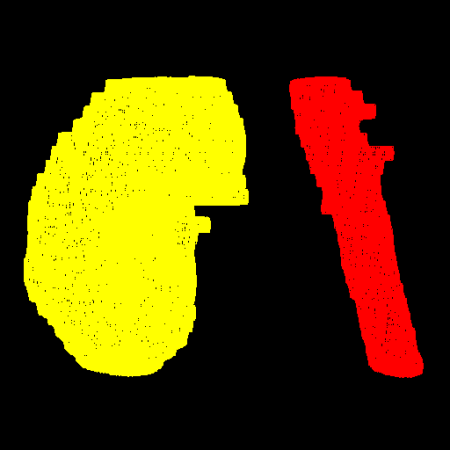
Figure 8 shows an example image.
 |
| Figure 8 |
Summary
In this article, we have seen the first stage of the mutliple material marching cubes algorithm for generating meshes from labelled volumes. As can be seen in the example image (which shows a portion of the right kidney and aorta), the output is a bit crude at this stage (and note that we're only able to render a smaller mesh), but the results are still quite good. In the next article, I'll explain the remainder of the algorithm, namely how to smooth and decimate the results to make the rendering of larger, nicer-looking meshes possible.
References
[Golodetz08] Golodetz, SM, 'Watersheds and Waterfalls' (Parts 1 and 2), Overload 83/84, February/April 2008.
[Schroeder92] Schroeder, WJ, et al., Decimation of Triangle Meshes, 1992.
[Wu03] Wu, Z, and Sullivan Jr., JM, 'Multiple material marching cubes algorithm', International Journal for Numerical Methods in Engineering, 2003.
Notes:
More fields may be available via dynamicdata ..