Journal Articles
| Browse in : |
All
> Journals
> Overload
> 83
(8)
All > Topics > Programming (877) All > Topics > Design (236) Any of these categories - All of these categories |
Note: when you create a new publication type, the articles module will automatically use the templates user-display-[publicationtype].xt and user-summary-[publicationtype].xt. If those templates do not exist when you try to preview or display a new article, you'll get this warning :-) Please place your own templates in themes/yourtheme/modules/articles . The templates will get the extension .xt there.
Title: Watersheds and Waterfalls
Author: webeditor
Date: 12 February 2008 08:58:00 +00:00 or Tue, 12 February 2008 08:58:00 +00:00
Summary: An introductory look at segmenting images into regions using a landscape analogy.
Body:
Introduction
In my last two articles [Golodetz], I talked about template metaprogramming, something most people would regard as a relatively 'pure' programming subject. For that reason, I thought it would make a nice change to look at something more applied this time: image segmentation.
Computing is one of those fields that encompasses so many diverse topics that it's impossible to know about all of them in depth. As programmers, we know more or less how to code (although there's always room for improvement!), but beyond a certain point, merely knowing how to write code in a certain language isn't enough. Before we can sit down and start hacking, we need to know what to code: we need, in short, domain knowledge.
Over the course of your programming career, there will inevitably be moments when you are forced outside your comfort zone, when you are asked to do things for which you initially lack the technical knowledge to do a good job. When that happens, you have three choices:
- Give up. This could involve panicking and trying to get the job allocated to someone else, quitting, or otherwise finding creative ways to avoid making a substantive attempt at the problem. Winners don't do this. (Well, unless it's also a really boring and pointless job, in which case they probably quit before it got to this point, anyway.)
- Fudge it. This is the 'it doesn't really matter if we do an inferior job as long as we get it out of the way' approach. It works quite well for problem sheets, but it's not the optimal approach to writing life-support code for the space shuttle. It's even more unprofessional than giving up and admitting that you don't know what you're doing.
- Learn. This involves looking upon your lack of knowledge as an opportunity. You can't possibly be expected to know everything about every possible subject. Being asked to do something unfamiliar is an excuse to expand what you know, giving you another tool in your armoury for the future. (Of course, some subjects are just genuinely hard, and may be beyond your mental capacity to comprehend them: if so, you may eventually have to reluctantly go to 1, but it's worth keeping at it for as long as possible first. You'd be surprised at what you can understand if you really try.)
During the course of my doctoral research at Oxford, I've found myself making this very choice numerous times. Whilst learning your way out of a problem is clearly the right way forward, it's not always easy: my most recent stumbling block, image processing, is only the latest in a long line of things which I've initially found it difficult to get to grips with. If you're faced with a difficult learning problem, then, the following tips might come in handy:
- Focus in on exactly what it is you're trying to find out - you can't learn about the whole field all at once.
- Don't get bogged down by reading papers which you don't understand - there's a reason you don't understand them. Either you don't have the prerequisite knowledge to understand them (most of the time) or they're badly written (some of the time), but either way, stubbornness will get you nowhere. Spend your time more productively by finding a different paper which explains things more clearly.
- Try and work out exactly what it is about an algorithm you don't understand - it's rarely the case that you understand 'absolutely nothing' about something. Identify the gaps in your knowledge and read as many papers (or other sources) as it takes to try and plug them. (This doesn't always have to be large numbers of papers - a few good papers will do just fine.)
- Start by trying to understand an algorithm at a high-level, then gradually focus in on the details. The lowest-level stage generally involves a pen and paper. (Incidentally, a pen and paper really does tend to be more effective for this stage than a computer. Don't make the mistake of substituting typing for thinking.)
- Once you think you've got something, try writing it out clearly in your own words or explaining it to someone who doesn't know anything about it. This is a good way to identify the bits you still don't quite get.
Ultimately, the efficacy of these methods is best demonstrated by the fact that until recently, the amount I knew about image processing could have been written on the back of a postage stamp! There's rarely a bad time to learn about something new...
The segmentation problem
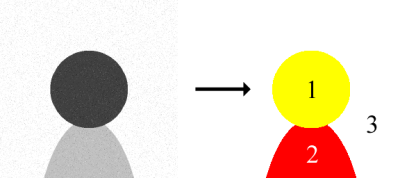
Image processing is itself a large field, so we're going to focus on one problem in particular, that of segmenting images. The idea is to classify the pixels of the image into different regions (see Figure 1 for a very simple example). This is important for the medical imaging work I'm doing because it allows relevant organs to be identified on the images; the results can then be used for further processing, e.g. for building 3D visualizations of the organs.
|
| Figure 1 |
There are numerous different approaches to the problem [Varshney], but the one I want to look at in particular is a method from the field of mathematical morphology called the watershed transform.
The landscape analogy
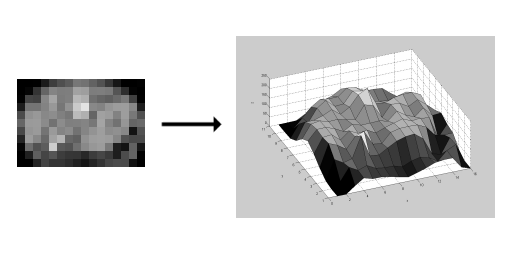
Anyone who's ever tried writing a terrain renderer will be familiar with the concept of using a heightmap to represent a landscape. Essentially, you have a 2D array of values, which can be viewed as an evenly-spaced finite grid located in the (x,y) plane. Each value represents the z height of the landscape at that point. (More formally, we could say that we have a rectangular domain Ω⊂ Z2 and a function f: Ω→ Z which gives the height of the landscape for every point in Ω.)
The insight behind the watershed transform is that a grey-scale image is nothing but such a 2D array of values, so it can be viewed as a landscape, where the heights are given by the grey levels in the image (see Figure 2).
|
| Figure 2 |
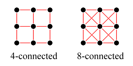
We now define a few terms. A pixel p ∈Ω has height f(p) and neighbour set N(p), according to some implementation-specific definition of neighbourhood (usually pixels are considered to be either 4-connected or 8-connected: see Figure 3).
|
| Figure 3 |
A singular minimum of the image is a point whose neighbours are all strictly higher than it. (More formally, p is a singular minimum if for all p′ ∈ N(p), f(p′) > f(p).) A plateau of the image is a maximal set of (two or more) connected pixels of equal altitude. A minimal plateau is a plateau from which it is impossible to descend, and a non-minimal plateau is the opposite. Together, the singular minima and minimal plateaux of the image form the regional minima of the image.
Flooding the image landscape
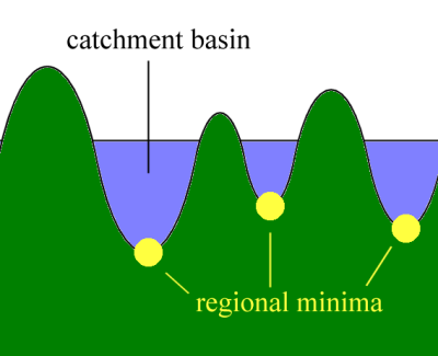
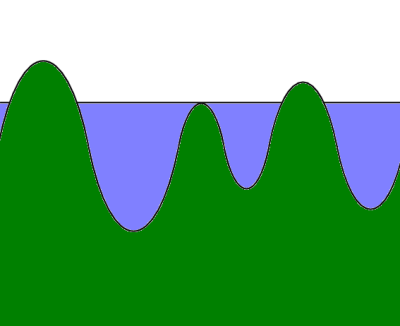
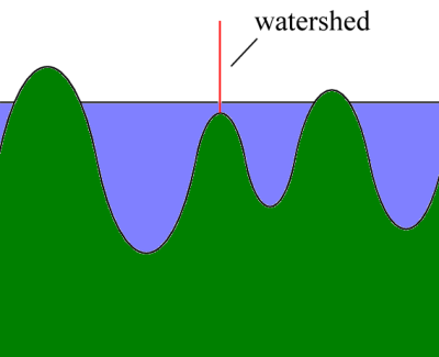
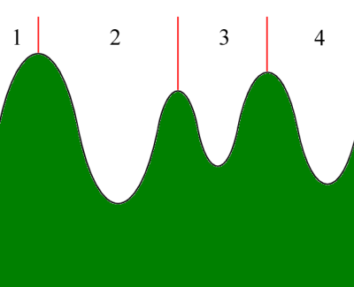
Imagine poking holes in the landscape at each of its regional minima, then lowering the landscape slowly into a lake. As the water begins to rise, pools of water will gradually form at each of the minima (see Figure 4). For reasons which will become obvious later, we'll call each pool of water the catchment basin of its associated minimum. If the water keeps rising, eventually some of the catchment basins will meet (see Figure 5): at this point, we imagine constructing a dam, or watershed, to keep them apart (see Figure 6) and continue the flooding. When the landscape has been fully flooded, the dams we've created will separate the different regional minima from each other at the points where their catchment basins would have met, thus segmenting the image into a number of regions, each associated with a different regional minimum (see Figure 7).
| Viewing an image as a landscape |
|
| Figure 4 | |
| Two catchment basins meet |
|
| Figure 5 | |
| Building a dam at the join point |
|
| Figure 6 | |
| The final division into regions |
|
| Figure 7 | |
This all sounds fine in theory, but there are a number of problems to be overcome:
- There's no reason to suppose that the things we want to segment (e.g. organs in a medical image) will have low grey levels and thus be in a 'valley'. If they are on top of a 'hill', we're apparently stuffed.
- The idea of the algorithm is one thing, but implementing it from this definition is far from straightforward.
- Images can have large numbers of regional minima, especially in the presence of noise. Most of them are irrelevant, but the end result is that the image will end up being greatly oversegmented.
Using the gradient image
The first problem is definitely image-specific. However, for medical images, we're helped greatly by the fact that the organs we're segmenting (e.g. the kidneys and liver) tend to be relatively homogeneous, i.e. the grey levels are relatively similar throughout the organ. This implies that the image landscape is relatively flat over each organ, or in other words that the gradient is small there. By contrast, the gradient at the edges of organs will, we hope, be quite large. By using the gradient of the original image, then, instead of the image itself, we engineer a situation where the things we're trying to segment are (by and large) in the valleys of the image, and are (more or less) surrounded by hills (see Figure 8).
| In the gradient image, homogeneous features of interest end up in the valleys |

|
| Figure 8 | |
Rainfall simulation
Implementing the algorithm using a flooding method is only one way of approaching the problem. It's certainly possible to implement it that way (e.g. [Rambabu]), but it's sometimes helpful to think about things from a different perspective. Instead of thinking of the watershed process as one of flooding, we can now imagine rain falling on each point of the landscape from above.
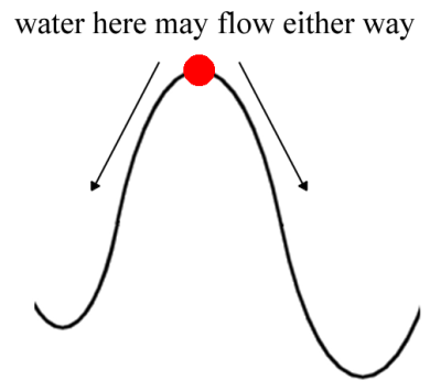
Water is notorious for taking the path of least resistance, and in this case that means running downhill to a regional minimum via a path of steepest descent (i.e. a path where at each stage we choose to move to a lowest neighbour of the current point). This gives us an idea for an alternative approach to the watershed transform: we can think of the catchment basin of a regional minimum as including all points whose unique path of steepest descent leads to the minimum in question. Where a point has more than one path of steepest descent, it can be allocated to any of the resulting minima according to programmer preference (see Figure 9).
| The flow direction at a point is ambiguous if it has more than one path of steepest descent |
|
| Figure 9 | |
Dealing with non-minimal plateaux
A problem occurs when we think about which way water should run off a non-minimal plateau. There are various different approaches to dealing with this [e.g. Bieniek; Osma-Ruiz; Stoev]; for the purposes of this article, we're going to use the approach in [Meijster] and transform the image to remove all non-minimal plateaux at the outset, thus making it what is called lower-complete.
In essence, the idea is to raise all plateau pixels up by their distance from the plateau edge (see Figure 10a). Of course, doing this naively doesn't work, since we might end up changing the ordering of the plateau pixels with respect to the other pixels in the image (see Figure 10b). The solution, then, is to find the maximum amount by which we're going to raise a plateau pixel and multiply the base image by that before raising any pixels on the plateau: this has the effect of 'spreading the landscape out' to accommodate the new altitudes in the middle (see Figure 10c).
| a) The 'intuition' is to raise plateau pixels by their distance from the edge |

|
| b) Doing this naively changes the height ordering of pixels in the image |

|
| c) This can be fixed by 'spreading the landscape out' prior to raising the pixels |

|
| Figure 10 | |
Implementing this is relatively straightforward using a queue (see Listing 1, building a lower-complete function). The basic idea is to add all pixels with a lower neighbour to the queue at the start, then gradually flood out from them a level at a time (essentially a breadth-first search), incrementing the distance counter after each level.
    Build-Lower-Complete(Function<Ω,Z> image)

    Function<Ω,Z> lc;
    Queue<PixelCoords> queue;
    // A marker indicating when we need to increase
    // the distance value.
    PixelCoords marker(-1,-1);
    // Initialise the queue with pixels that have a
    // lower neighbour.
    foreach(PixelCoords p ∈ Ω) {
      lc(p) = 0;
      foreach(PixelCoords neighbour ∈ N(p)) {
        if(image(neighbour) < image(p)) {
          queue.push(p);
          // To prevent it being queued twice.
          lc(p) = -1;
          break;
        }
      }
    }
    // Compute a function which indirectly indicates
    // the amount by which we need to raise the
    // plateau pixels (see the referenced paper for
    // more details).
    int dist = 1;
    queue.push(marker);
    while(!queue.empty()) {
      p = queue.pop();
      if(p == marker) {
        if(!queue.empty()) {
          queue.push(marker);
          ++dist;
        }
      }
      else
      {
        lc(p) = dist;
        foreach(PixelCoords neighbour  N(p)) {
          // If the neighbouring pixel is at the
          // same altitude and has not yet been
          // processed.
          if(image(neighbour) == image(p) &&
             lc(neighbour) == 0)
          {
            queue.push(neighbour);
            // To prevent it being queued twice.
            lc(neighbour) = -1;
          }
        }
      }
    }
    // Compute the final lower-complete function.
    // Note that at this point, dist holds the
    // amount by which we want to multiply the base
    // image.
    foreach(PixelCoords p ∈ Ω) {
      if(lc(p) != 0) {
        lc(p) = dist * image(p) + lc(p) - 1;
      }
    }
    return lc;
|
| Listing 1 |
Fletching
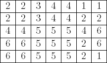
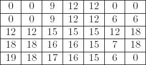
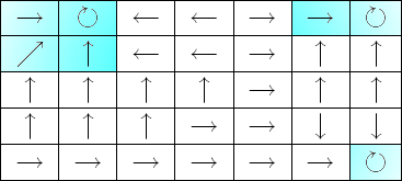
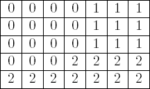
Having constructed a lower-complete image (see Figure 11b), the rest is all downhill (excuse the pun). Our next step is to construct an arrow on each node (see Figure 11c). In the case of a regional minimum, the arrow is a self-loop back to the node itself (for a minimal plateau, one of the nodes is chosen as a canonical element of the plateau and all the other nodes point to it); for all other nodes, the arrow points to a lowest neighbouring node (i.e. it points in the direction of a path of steepest descent). We also take the opportunity to numerically label all the canonical elements during this phase of the process.
| a) The original image |
|
| b) The lower-complete image |
|
| c) The arrows on each node |
|
| d) The final labelling |
|
| Figure 10 | |
The implementation (see Listing 2, constructing arrows on the nodes) uses an interesting disjoint-set forest data structure which I'll talk about in more detail next time. The idea is to combine all the minimum points into their respective regional minima using this data structure, and make all the other non-minimal points point to one of their lowest neighbours.
    Construct-Arrows(Function<Ω,Z> lc)

    Function<Ω,PixelCoords> arrows;
    Function<Ω,PixelCoords> labels;

    // Add all the minimum points to a disjoint set
    // forest.
    int labelCount = 0;
    DisjointSetForest<PixelCoords> minima;

    foreach(PixelCoords p ∈ Ω) {
      if(lc(p) == 0) {
        labels(p) = labelCount++;
        minima.add_node(p);
      }
    }

    foreach(PixelCoords p ∈ Ω) {
      if(lc(p) == 0) {
        // Union any neighbouring minimum points
        // into the same regional minimum.
        foreach(PixelCoords neighbour ∈ N(p)) {
          if(lc(neighbour) == 0) {
            minima.union_nodes(labels(p),
                               labels(neighbour));
          }
        }
      }
      else {
        // Find a lowest neighbour and make this
        // point's arrow point to it.
        PixelCoords lowestNeighbour(-1,-1);
        int lowestNeighbourValue = INT_MAX;

        foreach(PixelCoords neighbour ∈ N(p)) {
          if(lc(neighbour) < lowestNeighbourValue) {
            lowestNeighbour = neighbour;
            lowestNeighbourValue = lc(neighbour);
          }
        }

        // There will always be a lowest neighbour
        // here since the function's lower-complete.
        arrows(p) = lowestNeighbour;
      }
    }

    // Assign new labels to the canonical points of
    // the regional minima and make the arrows of
    // the non-canonical points point to them.
    labelCount = 1;
    foreach(PixelCoords p ∈ Ω) {
      if(lc(p) != 0) continue;
      int root = minima.find_set(labels(p));
      if(root == labels(p)) {
        // This is a canonical point.
        arrows(p) = p;
        labels(p) = labelCount++;
      }
      else {
        arrows(p) = minima.value_of(root);
      }
    }

    return (arrows, labels);
|
| Listing 2 |
Labelling the image
The final step of the basic watershed algorithm is to label the pixels (see Listing 3, labelling all the pixels by following the arrow chains). This involves following the arrows for each pixel to find which minimum it's associated with, and giving it the same label as that minimum. To speed things up, we use path compression when following a path to a minimum (i.e. we make all the arrows on the path point to the minimum once we've found it). Interestingly, this bears many similarities to the implementation of the disjoint-set data structure I just mentioned: we'll see more of this next time.
      Resolve-All(Function<Ω,PixelCoords> arrows,
                  Function<Ω,Z> labels)
      foreach(PixelCoords p ∈ Ω) {
        Resolve-Pixel(p, arrows, labels);
      }

      Resolve-Pixel(PixelCoords p,
                    Function<Ω,PixelCoords> arrows,
                    Function<Ω,Z> labels)

      PixelCoords parent = arrows(p);
      if(parent != p) {
        parent = Resolve-Pixel(parent);
        labels(p) = labels(parent);
      }
    return parent;
|
| Listing 3 |
The result (see Figure 11d) is, in general, an oversegmented image on which further processing is then required.
Pride comes before a 'fall
At this stage, we can be tolerably pleased with our efforts. We've managed to segment the image into a number of regions, each associated with a regional minimum of the image, but we haven't yet got what we need. In particular, our image is greatly over-segmented, because most of the regional minima aren't 'relevant': they're not associated with the objects of interest in our image. A general method to solving this problem involves trying to merge some of the regions together to reduce the overall number of regions in our image and obtain a better segmentation. One algorithm which takes this approach is the waterfall algorithm described in [Marcotegui], which I'll talk about next time. In and of itself, this still won't give us what we need for medical images, but it will take us a little closer to where we need to be. It also produces reasonable results on some non-medical images (e.g. the ones used in the paper). To get acceptable results for medical images, we have to make use of anatomical knowledge to process the results of application-independent algorithms like the waterfall, but that's something that is very much still a work in progress! Till next time...
References
[Bieniek] 'An efficient watershed algorithm based on connected components', Andreas Bieniek and Alina Moga; Albert-Ludwigs-Universitt Freiburg; Pattern Recognition 33 (2000) pp. 907-916
[Golodetz] 'Functional Programming Using C++ Templates (Parts 1 and 2)'; Overload 81 and Overload 82
[Marcotegui] Fast Implementation of Waterfall Based on Graphs, B. Marcotegui and S. Beucher; Ecole des Mines de Paris
[Meijster] A Disjoint Set Algorithm for the Watershed Transform, Arnold Meijster and Jos B. T. M. Roerdink, University of Groningen
[Osma-Ruiz] 'An improved watershed algorithm based on efficient computation of shortest paths', Víctor Osma-Ruiz et al., Universidad Politecnica de Madrid; Pattern Recognition 40 (2007) pp. 1078-1090
[Rambabu] 'An efficient immersion-based watershed transform method and its prototype architecture', C. Rambabu and Indrajit Chakrabarti; Journal of Systems Architecture 53 (2007) pp. 210-226
[Stoev] RaFSi - A Fast Watershed Algorithm Based on Rainfalling Simulation, Stanislav L. Stoev, University of Tübingen
[Varshney] Abdominal Organ Segmentation in CT Scan Images: A Survey, Lav R. Varshney, Cornell University
Notes:
More fields may be available via dynamicdata ..